Yes, I did just mix English, Spanish and French. And no, I am not living the “fishy” life, popular opinion to the contrary. Here’s the story. As someone who spends the majority of his time working online, with no oversight, I notice that I tend to drift a lot. I don’t play solitaire, or farm for virtual carrots, but I do wander over to Reddit more than I should, or poke around in this or that market in virtual assets to see if anything interesting has shown up. To some extent this can be justified. Many, perhaps all, of my profitable ventures have come from keeping my eyes open, poking around, doing my best to understand the digital world. On the other hand, at times I feel like I’ve been drifting aimlessly, that I’m all drift and no focus. My existing projects are gathering dust while I chase after shiny new things.
That’s the feeling, anyway. What does the evidence say? To keep track of what I was really doing, and perhaps nudge me towards more focus, I set a stopwatch to go off every 15 minutes. When it did, I would stop, write down what I was doing at that moment, and continue on. Perhaps you can see how these set intervals might provide an incentive to, shall we say, cheat? Especially right after the stopwatch chimed, I knew that whatever I did for the next few minutes was “free”, untracked. So I decided that I would have to write down everything I did during those 15 minute intervals, which worked sometimes, othertimes not so well.
My current solution? Setup a bell which chimes at random intervals, with an average time between chimes of 15 minutes. To hear what the bell sounds like, Go ahead and try it out, I think you’ll find it makes a nice sound. Leave that page open while you read the rest of this post, see how many times it rings.
At any rate, in order to randomize how long the wait was between chimes, I used a little something called a Poisson process. Actually, what I used was the Binomial approximation to the Poisson built from multiple Bernoulli trials, which results in wait times that are Exponential. Wait! Did you get all that? If so, then skip ahead until things look interesting. Otherwise, here’s more detail about how this works:
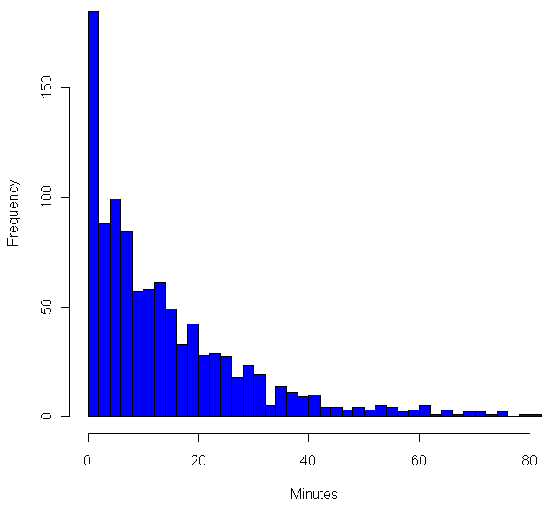
In order to determine the length of time between chimes, my computer generates a random number number between 0 and 1. If this random number is less than 1/15, then the next chime is in just one minute. Otherwise, the computer generates another random number and adds one minute to the time between chimes. On average, it will take 15 tries to get a number below 1/15, so the average time between chimes will be 15 minutes. However, to call 15 minutes the average is somewhat misleading. Here are the frequencies of different wait times (source code in R at the end):

As you can see, the most common time between chimes is just one minute. Strange, no? What’s going on here is that each test to see if the random number is below 1/15 is a Bernoulli trial, which is basically Italian for “maybe it succeeds, maybe it fails”. In this case “success” has probability of 1/15, failure happens the other 14 out of 15 times. In cases where probability is small, and you end of doing a lot of trials, the total number of successes over a given time period will have the Poisson distribution. The “Poisson” here is a Frenchman, who may or may not have smelled like his surname, but who certainly understood The Calculus as well as anyone in the early 1800’s. To get an even better approximation of the Poisson, I could have used trails with probability of success of 1/900, then treated each failure as another second of waiting time. That would have made the graph above smoother.
But wait! I didn’t show you a graph of the Poisson. I showed you a graph of something that approximates the exponential distribution. The number of chimes per hour is (roughly) Poisson distributed, but the waiting time between each chime is exponential, which means shorter wait times are more frequent, but no length of time, no matter how long, can be ruled out. In fact, the exponential distribution is the only (continuous) distribution which is “memoryless”. If you have waited 15 minutes for a chime, your expected wait time is still…. 15 minutes. In fact, your expected wait is independent of how long you have waited so far. The exponential distribution is a “maximal entropy” distribution, entropy in this case is related to how much you know. With the exponential, no matter how long you’ve waited, you still don’t know anything more than when you started waiting.
If you’ve been tuning out and scanning this post, now would be a good time to tune back in. I promise new and interesting things ahead!
It’s one things to understand the memoryless property of the exponential, even down to the mathematical nitty-gritty. It’s quite another to actually live with the exponential. No matter how well I know the formulas, I can’t shake the felling that the longer I have waited in between bell rings, the sooner the next chime must be coming. Certainly, it should be due any time now! While I “know” that any given minute has exactly the same probably as the next to bring with it the bell, the longer I wait, the nearer I feel the the next chime must be. After all, the back of my mind insists, once the page loads the wait time has been set into stone. However it was distributed before, it’s now a constant. Every minute you wait you are getting closer to the next bell, whenever it might have been set to come. I keep wanting to know more than I did a minute ago about about when the next bell will arrive.
This isn’t the only way in which I find my psyche battling with my intellect. I would also swear that over time the distribution of short waits and long waits evens out. Now, by the law of large numbers, it’s true that the more chimes I sit through, the closer the mean wait time will approach 15 minutes. However, even if you’ve just heard three quick bells in a row, that has absolutely no bearing on how long the wait will be between the next three chimes. The expected wait times going forward are completely independent of the wait times in the past. The mean remains 15 minutes, the median remains 10.4 minutes. Yet that’s not what I feel is happening, and over the past two weeks of experimenting with this I would swear that on days when there are a number of unusually quick intervals, these have been followed, later that very the same day, with unusually long intervals. And vice versa. It feels like things are evening out.
It’s possible that when my computer wakes up from a sleep mode, my web browser doesn’t remember where it was in a countdown to refreshing the chime page. So I reload it. Now, in theory, if you “reload” an exponential wait time while in process, this has absolutely no effect on your eventual wait time until the next chime. Yet anytime I reload the page, I have a moment of doubt as to whether I’m “cheating” in some way, to make what would have been a long wait shorter. In this case, the back of my mind says the exact opposite of its previous bias: because I am reloading a page that has been waiting a long time, this means that the wait time would have been really long. By starting the process anew, I’m increasing the chances of a short chime time.
Before you call me a nut, try living for a while with the timer running the background. Keep track of what you are doing if you want (and BTW I’ve found this to be every enlightening and more than a little sad), but mostly keep track of how you feel about the timing. Try reloading the page if you don’t hear a chime for a while. How does that feel? I suspect that in some ways humans were very well hard wired to understand probabilities. Yet I also suspect our wiring hinders how we understand probability, a suspicion backed up by all those gamblers out there waiting for the lucky break that’s well overdue.
CODE:
iters = 1000
results = rep(0,iters)
for (i in 1:iters) {
	minutes = 1
	while(runif(1)>(1/15)){
		minutes = minutes + 1
	}

	results[i] = minutes
}

hist(results, breaks=40, col="blue", xlab="Minutes")


