plot


1
Sep 14

Labor day distribution fun

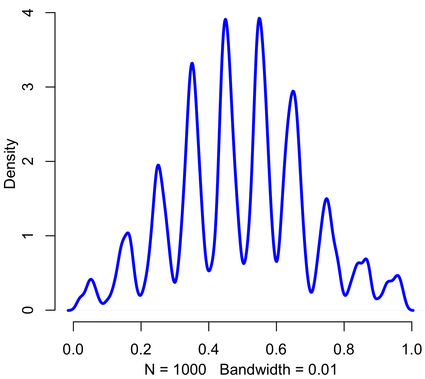
Pinned, entropy augmented, digitally normal distribution, of no particular work-related use and thus perfectly suitable for today. Code in R:

iters = 1000
sd = 2
precision = 20

results = rep(0,iters)

for(i in 1:iters) {
	x = floor(rnorm(20,5,sd) %% 10)
	results[i] = paste(c('.',x),sep="",collapse="")
}

results = as.numeric(results)

plot(density(results,bw=.01),col="blue",lwd=3,bty="n")

14
Dec 12

Let it snow!

A couple days ago I noticed a fun piece of R code by Allan Roberts, which lets you create a digital snowflake by cutting out virtual triangles. Go give it a try. Roberts inspired me to create a whole night sky of snowflakes. I tried to make the snowfall look as organic as possible. There are lots of options to adjust. Here’s the code, have fun and Happy Holidays!

# Code by Matt Asher for statisticsblog.com
# Feel free to modify and redistribute 

# How many flakes do you want to fall?
flakes = 100

# Width and height of your space
width = 800
height = 600

# Initial wind
wind = 0

# Setup the background of the plot and margins
par(bg = "black")
par(oma=c(0,0,0,0))
par(mar=c(0,0,0,0))
plot(0, 0, col="black", pch=".", xlim=c(0,width), ylim=c(0,height), axes=F)

for(i in 1:flakes) {
    startY = height
    startX = runif(1,1,width)

    xPos = startX
    yPos = startY

    for(j in 1:height) {

		# Optional drift in wind
		wind = wind + rcauchy(1,0,.05)

		# Update snowflake position
        xPos = xPos + rnorm(1,.1,1.5)
        yPos = yPos - runif(1,4,20)

        # Are we in the space, if so display it
        if(xPos > 0 && xPos <= width && yPos > 0 && yPos <= height) {
            points(round(xPos), round(yPos), col="white", pch=8)

            # System dely, slows down the flakes
            Sys.sleep(0.1)
        }
    }
}

25
Nov 11

Interactive map of US road fatalities


Fantastic map which shows the location of every death on US roads from 2001 to 2009. Go take a look then come back and tell me….

What location did you zoom in on first, and why?


19
Jul 10

R: Clash of the cannon cycles

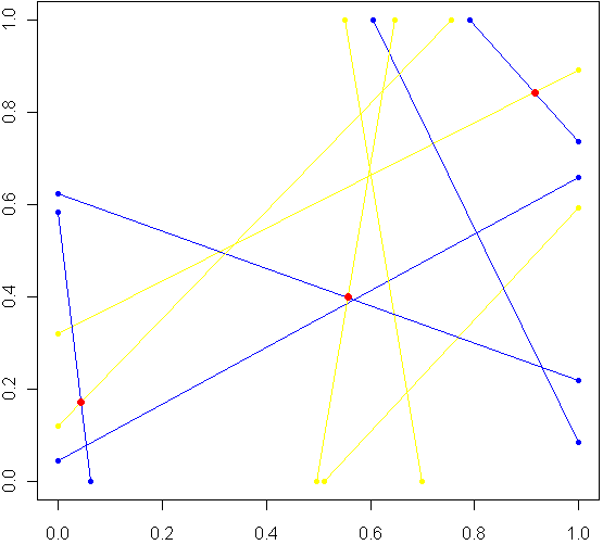
Imagine a unit square. Every side has length 1, perfectly square. Now imagine this square was really a fence, and you picked two spots at random along the fence, with uniform probability over the length of the fence. At each of these two locations, set down a special kind of cannon. Just like the light cycles from Tron, these cannons leave trails of color. To aim each cannon, pick another random point from one of the three other sides of the fence, and aim for that point.

Sometimes there will be a collision within the square, other times no. The image at top shows the results of five trials. The red dots are where the trails from a pair of cannons collided. My burning question: What is the distribution for these dots? Before reading on, try to make a guess. Where will collisions be most likely to happen?

Somewhere in the world, there lives a probabilist who could come up with a formula for the exact distribution in an hour, but that person doesn’t live in my house, so I took the Monte Carlo approach, coded in R:

# Functions to pick two points, not on the same side:
m2pt <- function(m) {
	if(m <1) {
		myPoint = c(5,m,0)
	} else if (m < 2) {
		myPoint = c(6,1,m %% 1) 
	} else if (m < 3) {
		myPoint = c(7,1-(m %% 1),1)
	} else {
		myPoint = c(8,0,1-(m %% 1))
	}
	return(myPoint)
}		

get2pts <- function() {
	pt1 = m2pt(runif(1,0,4))
	pt2 = m2pt(runif(1,0,4))
	
	# Make sure not both on the same sides. If so, keep trying
	while(pt1[1] == pt2[1]) {
		pt2 = m2pt(runif(1,0,4))
	}
	return(c(pt1[2:3],pt2[2:3]))
}

# Optional plot of every cannon fire line. Not a good idea for "iters" more than 100
#windows()
#plot(0,0,xlim=c(0,1),ylim=c(0,1),col="white")		
		
# How many times to run the experiment
iters = 10000

# Track where the intersections occur
interx = c()
intery = c()

for(i in 1:iters) {
	can1 = get2pts()
	can2 = get2pts()
	
	# Optional plot of every cannon fire line. Not a good idea for "iters" more than 100 
	#points(c(can1[1],can1[3]),c(can1[2],can1[4]),pch=20,col="yellow")
	#segments(can1[1],can1[2],can1[3],can1[4],pch=20,col="yellow",lwd=1.5)
	#points(c(can2[1],can2[3]),c(can2[2],can2[4]),pch=20,col="blue")
	#segments(can2[1],can2[2],can2[3],can2[4],pch=20,col="blue",lwd=1.5)

	# See if there is a point of intersection, find it. 
	toSolve = matrix(c( can1[3]-can1[1], can2[3]-can2[1], can1[4]-can1[2], can2[4]-can2[2]),byrow=T,ncol=2)
	paras = solve(toSolve, c( can2[1]-can1[1], can2[2]-can1[2]))
	
	solution = c(can1[1] + paras[1]*(can1[3]-can1[1]), can1[2] + paras[1]*(can1[4]-can1[2]))
	
	# Was the collision in the square
	if(min(solution) > 0 && max(solution) < 1) {
		# Optional plot of red dots
		# points(solution[1],solution[2],pch=20,col="red",cex=1.5)
		
		# if this intersection is in square, plot it, add it to list of intersections
		interx = c(interx, solution[1])
		intery = c(intery, solution[2])
	}
}

windows()
plot(interx, intery, pch=20,col="blue",xlim=c(0,1),ylim=c(0,1))

After carefully writing and debugging much more code than I expected, I ran a trial with several thousand cannon fires and plotted just the collisions. Here is what I saw:

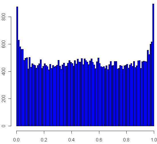
Looks pretty uniform, doesn't it? If it is, I will have gone a very long way just to replicate the bi-variate uniform distribution. My own original guess was that most collisions, if they happened in the square, would be towards the middle. Clearly this wasn't the case. Looks can be deceiving, though, so I checked a histogram of the x's (no need to check the y's, by symmetry they have the same distribution):

Very interesting, no? The area near the edges appears more likely to have a collision, with an overall rounded bowl shape to the curve. The great thing about Monte Carlo simulations is that if something unexpected happens, you can always run it again with more trials. Here I changed "iters" to 100,000, ran the code again, and plotted the histogram.

hist(interx, breaks=100, col="blue",xlab="x",main="Histogram of the x's")

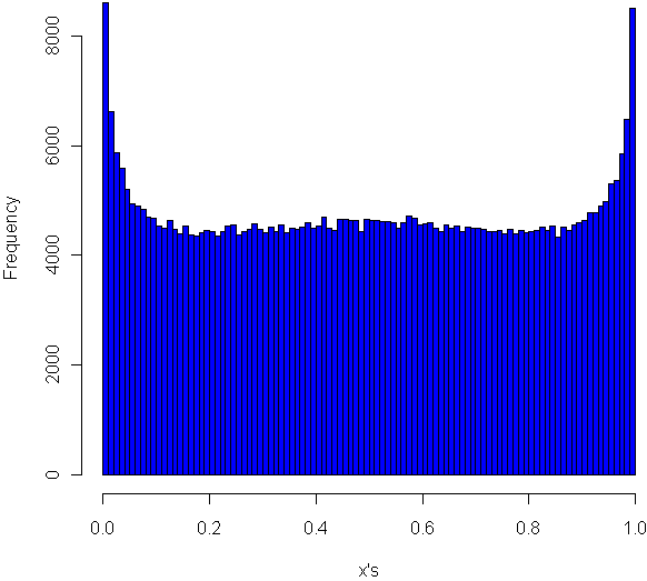
Now its clear that the distribution spikes way up near the edges, and appears to be essentially flat for most of the middle area. It seems like it may even go up slightly at the very middle. Just to be sure, I ran a trial with one million iterations:

Now it definitely looks like a small upward bulge in the middle, though to be sure I would have to do run some statistical tests or use an even larger Monte Carlo sample, and given how inefficient my code is, that could take the better part of a week to run. So for today I'll leave it at that.

One final statistic of note: During my run of one million iterations, 47.22% of all collisions happened inside the box. What do you think, is the true, theoretical ratio of collisions within the box a rational number?


2
Jul 10

Word games in probability and R

Last night, while playing Boggle, we ended up with a board without a single vowel. Not even a “Y” or “Qu”. This seemed fairly unusual, so I wondered what the chances were of such an occurrence. I found an online list of the letters each die has, and I could have written down the number of vowels on each one by hand, but whenever possible I like to do things by computer. So I fired up Hal and asked for some help with the calculations.

Apparently some European boards use a 5 x 5 grid, but here in the land of the Maple leaf our board has 16 cubes. Here are the letters on them, as I coded them into R:

d1 = c('S','R','E','L','A','C')
d2 = c('D','P','A','C','E','M')
d3 = c('Qu','B','A','O','J','M')
d4 = c('D','U','T','O','K','N')
d5 = c('O','M','H ','R','S','A')
d6 = c('E','I','F','E','H','Y')
d7 = c('B','R','I','F','O','X')
d8 = c('R','L','U','W','I','G')
d9 = c('N','S','O','W','E','D')
d10 = c('Y ','L','I','B','A','T')
d11 = c('T','N','I','G','E','V')
d12 = c('T','A','C','I','T','O')
d13 = c('P','S','U','T','E','L')
d14 = c('E','P','I','S','H ','N')
d15 = c('Y','K','U','L','E','G')
d16 = c('N','Z','E','V','A','D')

So now I had to check how many vowels were on each die. Here’s the code I used for this:

vowels = c('A','E','I','O','U','Qu','y')
vowelsFound = rep(0,16)
for(i in 1:16) {
	found = 0
	die = eval(parse(text=paste("d",i,collapse="",sep="")))
	for(l in die) {
		# Check to see if this letter is in the vowels vector
		if(l %in% vowels) {
			found = found + 1
		}
	}
	vowelsFound[i] = found
}

# Probabilities of getting a vowel for each die
pVowels = vowelsFound/6

# Probability of getting no vowel for each die
pNoVowels = 1 - pVowels

# Chance that we will get not a single vowel, including "y" and "Qu"
print(prod(pNoVowels))

If you run the code above, you should see that the probability of getting no vowels (including “Y” and “Qu”) is 0.000642. That works out to one in every 1557 boards. So it’s quite rare, but by no means so extraordinary that it crosses the Universal probability bound. Also, it’s not enough to just calculate how rare your event is, or how rare any similar or more extreme event is, and then be astounded. You also have to include all the other possible events that would have left you amazed. What about getting all vowels (much more rare)? What about getting 8 or 9 E’s, or a row or column of all A’s or E’s? It’s likely that if you add up all probabilities of all the rare events which might leave you amazed, you’ll end up with a good chance of amazement every time.

I could have stopped here, but having coded the dice, I decided to create a simplified version of the game in R. If I have a chance over the next few days I’ll add some more features.

# You will need to download a dictionary file. I found one here:
# http://svn.pietdepsi.com/repos/projects/zyzzyva/trunk/data/words/north-american/owl2-lwl.txt
words = read.table("wordlistData.dat", colClasses = "character")
words = unlist(words[,1])

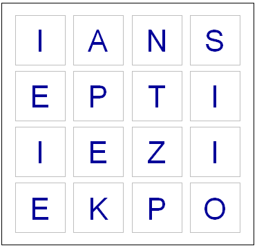
# Create a random board. Plot it.
board = diag(4)
dice = sample(1:16,16)
cntr = 4
for(i in dice) {
	die = eval(parse(text=paste("d",i,collapse="",sep="")))
	board[floor(cntr/4), (cntr %% 4) + 1] = sample(die,1)
	cntr = cntr + 1
}

plot(0,0,xlim=c(0,4),ylim=c(0,4),col="white",ann=FALSE, xaxt="n", yaxt="n" )

for(m in 1:4) {
	for(n in 1:4) {
		text(m-.5,n-.5,labels=board[m,n],cex=2.75,col="#000099")
		# Draw a square the easy way
		points(m-.5,n-.5,pch=0,cex=10,lwd=1.5,col="gray")
	}
}

# How many seconds to give for each round
gameTime = 180

START_TIME = proc.time()[3]	
elapsed = 0

# Simple scoring, with 1 point per letter. 
# Dictionary only has words length 3 or longer
score = 0

cat("Find words. Hit enter after each word.\n")
while(elapsed < gameTime) {
	myWord = scan(n=1, what=character()) # Get a single word
	elapsed = signif(proc.time()[3] - START_TIME, digits=4)
	if (length(myWord)==0) {
		cat("You have", gameTime - elapsed, "seconds left. Keep going!\n")
	} else {
		
		if(elapsed < gameTime) {
			# Check if it's a real word, see if it is in dictionary
			# Convert their guess to uppercase letter
			myWord = toupper(myWord)
			
			# If it is in the dictionary, give them points
			if(myWord %in% words) {
				# Make sure they haven't used this word before TODO
			
				# Add it to their score
				score = score + nchar(myWord)
				cat("Congratulations. You are up to", score, "points.")
				cat("You have", gameTime - elapsed, "seconds left. Keep going!\n")
			} else {
				# If it isn't in the dictionary, let the user know that they got it wrong.
				cat("Sorry, that is not in the dictionary. Keep trying!\n")
			}
			
			
		}
	}
} 

cat("Out of time! ")
cat("Your final score was:", score, "points.")

Enjoy the game. Let me know if you notice any issues or have suggestions!


14
Jun 10

Repulsive dots pattern, the difference of distance

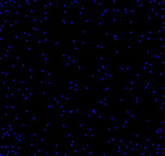
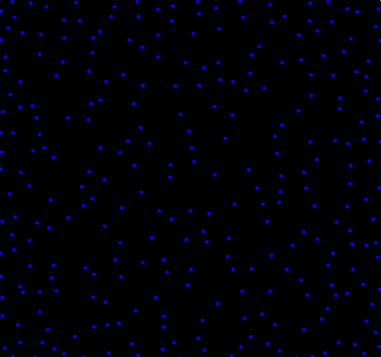
What if you wanted to randomly place objects into a field, and the more objects you had, the more they rejected newcomers placed nearby? To find out, I setup a simulation. The code, shown at the end, isn’t all that interesting, and the plots shown below aren’t all that special. I think there is one interesting part of this, and that’s how the clustering changes depending on how distance is measured. One of the plots uses the traditional “L2″ distance, the other uses L1” (Manhattan taxi cab) measure . Each plot shown below has almost exactly the same number of dots (277 vs 279). Can you tell which uses L1 and which uses L2 just by looking?

Plot A:

Plot B:

Here’s the code. Run it and see for yourself. Make sure to change adjust the values which have comments next to them. Uncommenting “print(force)” can help you pack a maxRepulse value.

calcRepulse <- function(x,y,dots,use="L2") {
	force = 0
	i = 1
	while(i <= dim(dots)[1] && dots[i,1] != 0) {
		if(use == "L2") {
			force = force + 1/( (x-dots[i,1])^2 + (y-dots[i,2])^2 )
		} else if(use == "L1") {
			force = force + 1/( abs(x-dots[i,1]) + abs(y-dots[i,2]) )
		}
		i = i+1
	}
	# print(force)
	return(force)
}

par(bg="black")
par(mar=c(0,0,0,0))
plot(c(0,1),c(0,1),col="white",pch=".",xlim=c(0,1),ylim=c(0,1))

place = 1 #Maximum number of dots to place, change this to something bigger
dots = matrix(rep(0,place*2),ncol=2)
maxTries = place * 10
maxRepulse = 1 # Anything above this will be rejected as too repulsive a location
dist2use = "" # Pick L1 or L2

placed = 0
tries = 0


while(placed < place && tries < maxTries) {
	x = runif(1)
	y = runif(1)
	
	if(calcRepulse(x,y,dots,dist2use) < maxRepulse) {
		dots[(placed + 1),1] = x
		dots[(placed + 1),2] = y
		placed = placed + 1
		points(x,y,col="blue",pch=20)
	}

	tries = tries + 1
}

28
May 10

R: More plotting fun with Poission

Coded as follows:

x = seq(.001,50,.001)
par(bg="black")
par(mar=c(0,0,0,0)) 
plot(x,sin(1/x)*rpois(length(x),x),pch=20,col="blue")

3
May 10

First annual R plot replication prize

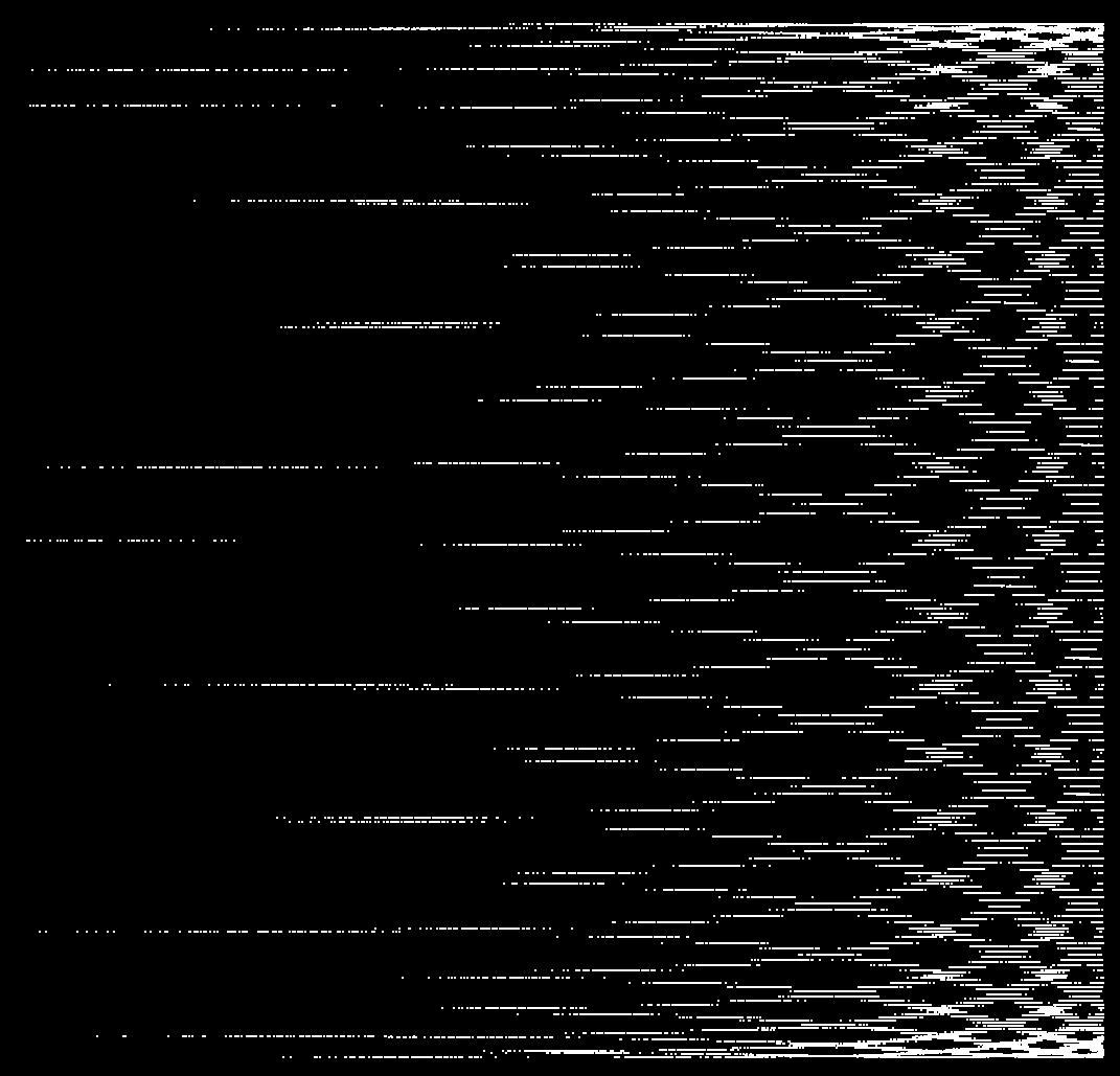
Click image for the full-size version

$100 to the first person who can figure out how I created this plot and replicate it. Some hints:

  • It was done in R.
  • There is only one underlying probability distribution involved (one “rdist()“).
  • Including the “plot” statement, I created this with 3 short lines of code.

This is based on a random sampling of unstated size, so I don’t expect that your graph will be an absolute, exact match.

I’ll add $1 to the prize for every day that goes by without a winner until the end of the year. After that I’ll consider it an unsolved mystery and reveal the code I used.

Post your guesses for the code as a comment to this post. First correct answer wins. Good luck to all!


21
Apr 10

R: more plotting fun, this time with the Poisson

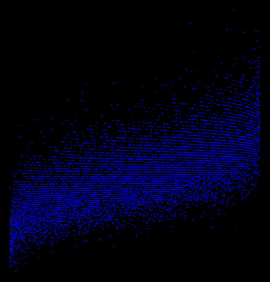
Click on image for a larger version. Here is the code:

par(bg="black")
par(mar=c(0,0,0,0)) plot(sort(rpois(10000,100))/rpois(10000,100),frame.plot=F,pch=20,col="blue")  

8
Apr 10

R: another nifty graph

Make sure to click on the image to see the large version. Code for this graph:

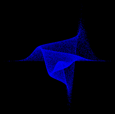
moxbuller = function(n) {   
	u = runif(n)   
	v = runif(n)   
	x = cos(2*pi*u)*sqrt(-2*log(v))  
	y = sin(2*pi*v)*sqrt(-2*log(u))
	r = list(x=x, y=y)
	return(r) 
}
r = moxbuller(50000) 
par(bg="black") 
par(mar=c(0,0,0,0)) 
plot(r$x,r$y, pch=".", col="blue", cex=1.2)