Usually when you are doing Monte Carlo testing, you want fake data that’s good, but not too good. You may want a sample taken from the Uniform distribution, but you don’t want your values to be uniformly distributed. In other words, if you were to order your sample values from lowest to highest, you don’t want them to all be equidistant. That might lead to problems if your underlying data or model has periods or cycles, and in any case it may fail to provide correct information about what would happen with real data samples.
However, there are times when you want the sample to be “perfect”. For example, in systematic sampling you may wish to select every 10th object from a population that is already ordered from smallest to biggest. This method of sampling can reduce the variance of your estimate without introducing bias. Generating the numbers for this perfect sample is quite easy in the case of the Uniform distribution. For example, R gives you a couple easy ways to do it:
# Generate a set of 100 equidistant values between 5 and 10 (inclusive)
x <- seq(5,10,length=100)

# Generate every 12th integer between 50 and 1000
x <- seq(50,1000,12)
When it comes to other distributions, grabbing a perfect sample is much harder. Even people who do a lot of MC testing and modeling may not need perfect samples every day, but it comes up often enough that R should really have the ability to do it baked right into to the language. However, I wasn't able to find such a function in R or in any of the packages, based on my searches at Google and RSeek. So what else could I do but roll my own?
# Function returns a "perfect" sample of size n from distribution myDist
# The sample is based on uniformly distributed quantiles between 0 and 1 (exclusive)
# If the distribution takes additional parameters, these can be specified in the vector params
# Created by Matt Asher of StatisticsBlog.com
perfect.sample <- function(n, myDist, params = c()) {
	x <- seq(0,1,length=(n+2))[2:(n+1)]

	if(length(params)) {
	  	toEval <- paste(c("sapply(x,q", myDist, ",", paste(params,collapse=","), ")"), collapse="")
	} else {
	  	toEval <- paste(c("sapply(x,q", myDist, paste(params,collapse=","), ")"), collapse="")
	}

	eval(parse(text=toEval))
}
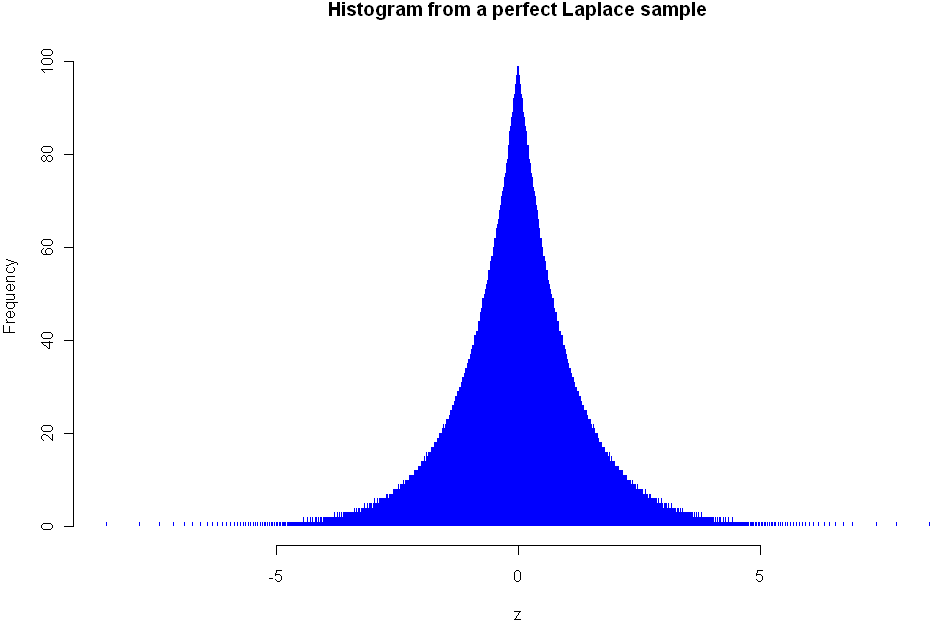
This function should work with any distribution that follows the naming convention of using "dname" for the density of the distribution and has as its first parameter the number of values to sample. The histogram at the top of this post shows the density of the Lapalce, aka Double Exponential distribution. Here is the code I used to create it:
# Needed library for laplace
library(VGAM)
z <- perfect.sample(5000,"laplace",c(0,1))
hist(z,breaks=800,col="blue",border=0,main="Histogram from a perfect Laplace sample")
As you can see, my function plays nice with distributions specified in other packages. Here are a couple more examples using standard R distributions:
# Examples:
perfect.sample(100,"norm")

# Sampling from the uniform distribution with min=10 and max=20
z <- perfect.sample(50,"unif",c(10,20))
Besides plotting the results with a histogram, there are specific tests you can run to see if values are consistent with sampling from a known distribution. Here are tests for uniformity and normality. You should get a p-value of 1 for both of these:
# Test to verify that this is a perfect sample, requires library ddst
# Note only tests to see if it is Uniform(0,1) distributed
library(ddst)
ddst.uniform.test(z, compute.p=TRUE)

# Needed for the Shapiro-Wilk Normality Test
library(stats)
z = perfect.sample(1000,"norm")
shapiro.test(z)
If you notice any bugs with the "perfect.sample" function please let me know. Also let me know if you find yourself using the function on a regular basis.

