Head down to your local hardware store and pick up a smoke detector. Pop off the cover and look inside. You’ll see a label that mentions Americium 241, a radioactive isotope. Put on your HEV suit, grab a pair of tweezers and a fine-tipped pen, and remove the 0.3 millionths of a gram of Americium. If you need reading glasses, now might be a good time to put them on. Pick out one of atoms and label it with an X. Now watch closely. Sooner or later, it will spit out an Alpha particle.
Just how long will you have to wait? Decay rates are measured in half-lives, which is the amount of time needed for half of the particles to decay (any particular atom has a 1/2 chance of decaying in this time as well). The stated half-life for this isotope is 432 years, and your waiting time will follow an exponential distribution. The strange, oddly beguiling quality about this distribution is that the conditional probabilities remains constant. In other words, no matter how long you’ve waited, there’s still a 1 in 2 chance that your Americium isotope will decay in the next 432 years. Waiting for an exponentially distributed event to happen leads to an odd feeling, at least for me. The longer you wait, the more you “expect” the event to happen soon, even knowing that your expected wait time never changes. I wrote about that feeling previously, and created an exponential timer you can try out for yourself. I would suggest setting it to less than 432 years.
Cranking uncertainty up to 11
Recently, as I waited patiently for my own particle of Americium to give up its Alpha, I got to thinking about conditional uncertainty. No matter how long we wait for our event, we never get any smarter about when it will happen. But we don’t get any dumber, either. Would it be possible, I wondered, to build a kind of “super-exponential” distribution, where the longer we wait, the less we know. In other words, can we take our level of uncertainty up to 11?
Imagine the following scenario: first we sample from a standard uniform distribution, which gives us a number somewhere between 0 and 1. Call this number [latex]U[/latex]. Then we take [latex]U[/latex] (without looking at it!), and plug it into the exponential distribution as the parameter [latex]\lambda[/latex]. This gives us a random variable with a mean waiting time of [latex]\frac{1}{U}[/latex] for the first occurrence. (Note that this mean isn’t the same as the half-life, which is actually the median. To convert from mean to half-life, multiply by the natural log of 2).
My prediction was that this method would increase the overall level of uncertainty about our waiting time, and, even worse, make our uncertainty grow over time. Why? The longer we’ve waited, I figured, the more likely our (presumed) [latex]\lambda[/latex] will be small, which in turn means the expectation and variance of our exponential waiting time grow, widening our confidence intervals.
At this point, I had the vague feeling that this probability distribution should already exist as a known thing, that it may even be a version of something I’ve encountered before. Another way to look at the exponential is in terms of the failure rate, or, conversely, the survival rate. When Ed Norton, the un-named narrator of Fight Club (I know, I know), says that “on a long enough timeline, the survival rate for everyone drops to zero,” this is what he means. Only Norton is referring to the cumulative survival rate, whereas it’s usually most interesting to look at the instantaneous (or marginal, for my economist friends) rate. For the exponential this rate is constant, ie flat. There is a distribution specifically crafted to let you simulate failure rates when the rate itself is variable, it’s called the Weibull. It can be used to model products whose expected durability increases with time (note that we are not saying the product becomes more durable over time, but that the fact that it has survived tells us that it is highly durable). Did I just rediscover the Weibull, or one it’s friends in the same family of extreme distributions?
Before breaking out my great big Compendium of Probability Distributions, I dove right in with a quick Monte Carlo simulation. As with all my posts using R, you’ll find the code at the end of this post.
A wave of plots
Here’s the histogram for our sample, with the rightmost tail chopped off (because your screen, unlike mine, is just too damn small):
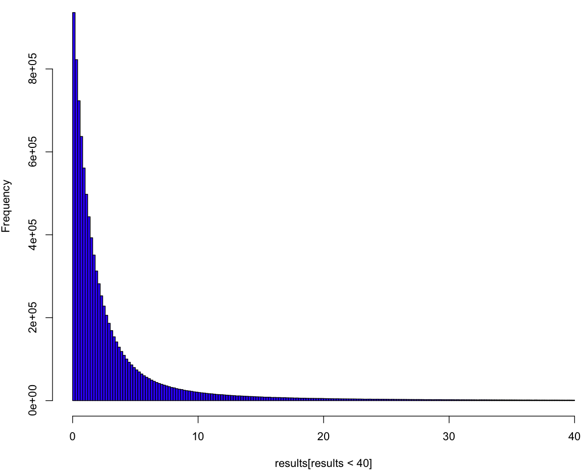
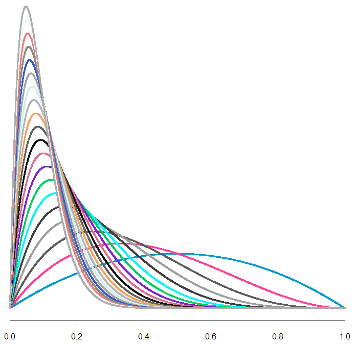
So it looks like a variant of the exponential, but this plot doesn’t tell us much. To really understand the distribution we have to see it as if we were inside the distribution, waiting for the event to happen. All we know is the process, and we have to come up with a guess about our distribution curve conditional on how long we’ve waited so far. In order to understand this curve, we first need to make a guess about [latex]\lambda[/latex], which is to say [latex]U[/latex]. Can we put a probability distribution on [latex]U[/latex] given how long we’ve been waiting so far? Yes, we most certainly can! And, because our prior distribution on [latex]U[/latex] is uniform (of course), our posterior is our likelihood. Here’s what our (posterior) curves look like:
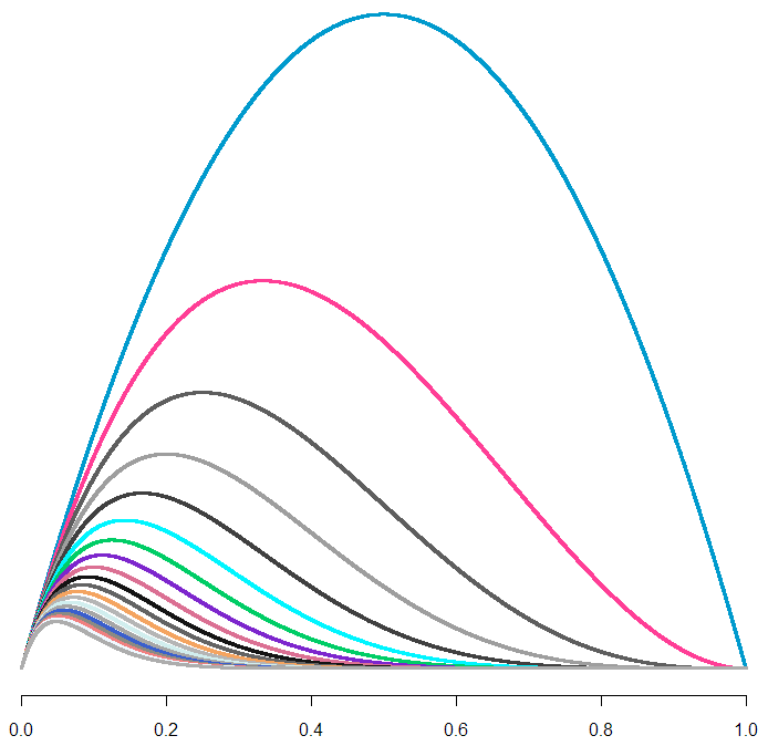
Each curve is a probability distribution on our belief about [latex]U[/latex]. In other words, the peaks represent what we believe to be the most likely value for [latex]U[/latex], given how long we’ve waited so far. The biggest curve is our distribution for [latex]U[/latex] after waiting for one unit of time (let’s just call them “minutes”). As you can tell, if we continue to wait, our maximum likelihood estimate (MLE) for [latex]U[/latex] shifts left, and it looks like our curve flattens out. But wait! Each of these curves has a different area. To treat them like a true probability distribution, we should normalize each of the areas to one. Here’s what those same curves look like after normalization:
From this handsome chart (the same one from the beginning of the post), we can tell that expected range of values for [latex]U[/latex] is narrowing, not broadening. So could our uncertainty be decreasing along with our wait, as we hone in on the true value of [latex]U[/latex]? Let’s take a look at what happens to our additional wait time as time passes.
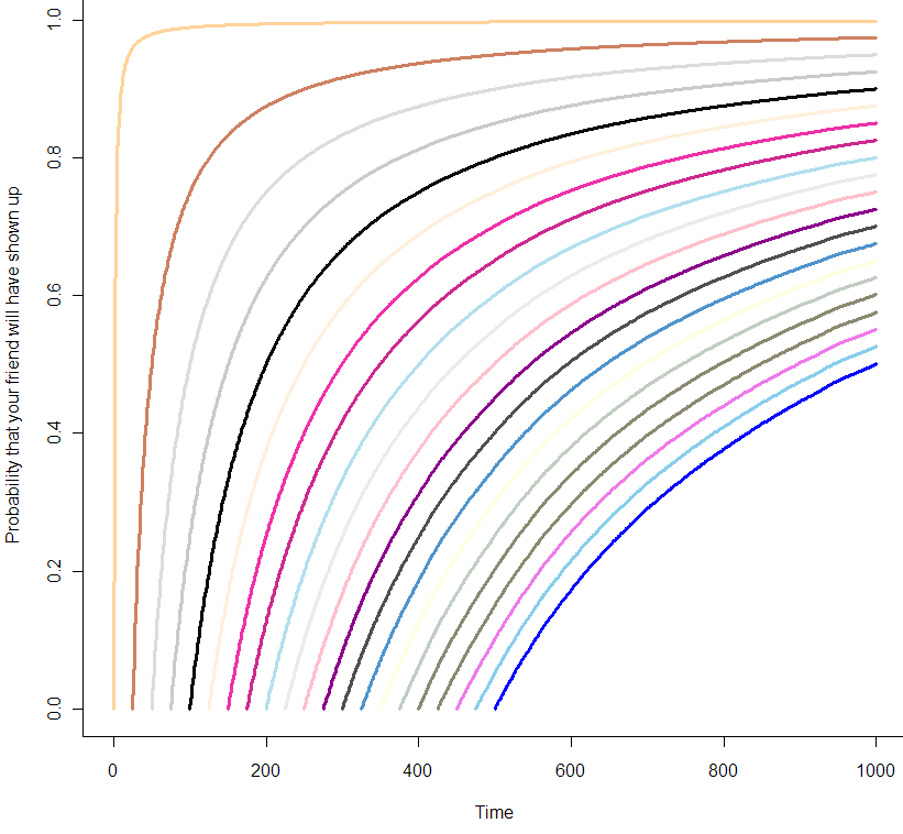
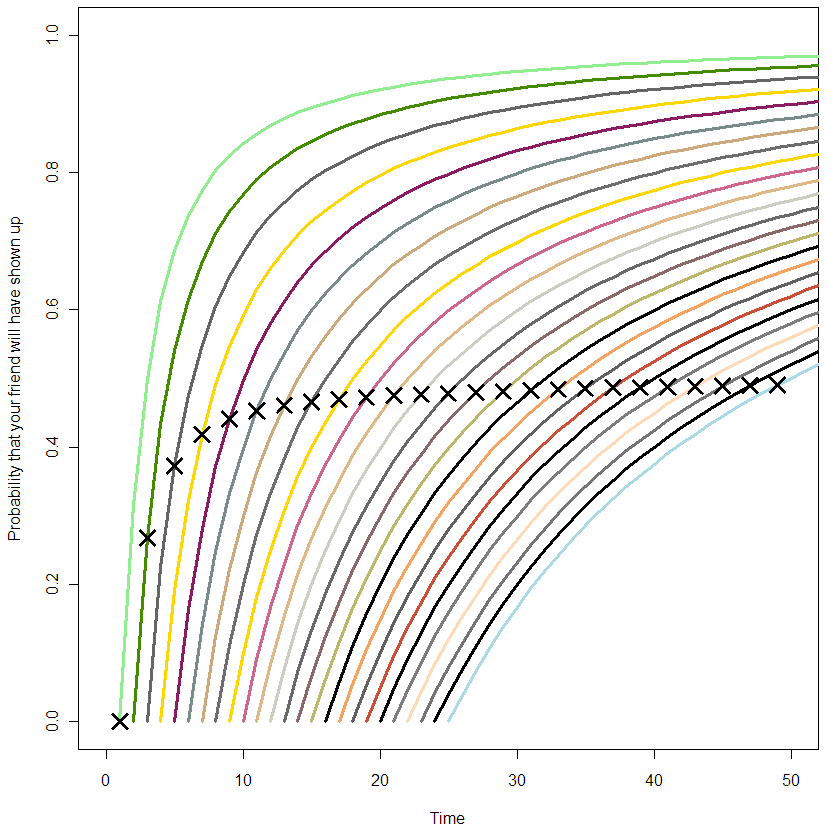
You can think of these curves as the chance that your friend will show up in the coming minutes, given how long you’ve already been waiting. At the very beginning of your wait, modeled by the orange curve at the far left, you can be almost certain that your friend will show up in the next 10 minutes. But by the time you’ve been waiting for 500 minutes, as seen in the blue curve at the far right, you are only 50% sure that she will show up in the next 500 minutes. Are those probabilities exact? It seems like it, but let’s zoom in on the first 25 minutes:
The X’s represent the median time for your friend’s arrival. If this was always equal to your wait time so far, all of the X’s would be in a straight line at 0.5. From this plot, it’s clear that this is not the case from the beginning, but only becomes so as you wait longer. So what have we got here? At this point I’m at the limit of what I can get out of Monte Carlo. It’s time to do math! (or not, feel free to skip this next section).
The formula
To get the pdf for this distribtion, I start by noting that if we had two possible choices for [latex]\lambda[/latex] with a one-half chance each of being picked, then the probability our waiting time would be less than [latex]x[/latex] would be:
[latex] P(t < x) = \frac{1}{2}(1 - e^{-x \lambda_1}) + \frac{1}{2} (1 - e^{-x \lambda_2})[/latex]
where [latex](1 – e^{-x \lambda_i})[/latex] is the cumulative distribution function (CDF) of the exponential distribution with parameter [latex]\lambda_i[/latex]. If you really know your exponential, you may have noticed some similarities with the hyperexponential distribution, but we’re gonna take it to the limit, and create a kind of hyper-hyperexponential. More generally, for a sample of [latex]\lambda_i[/latex]:
[latex]P(t < x) = \frac{1}{n} \sum_{i=1}^n (1 - e^{-\lambda_i x}) [/latex]
Since the [latex]\lambda_i[/latex] are uniformly distributed, the more of them we sample, the more our order statistics are going to look like [latex](\frac{1}{n}, \frac{2}{n}, \frac{3}{n}... \frac{n}{n})[/latex] where our sample size is n (proof is left as an exercise for you, my dear reader).
[latex]P(t < x) = \frac{1}{n}\sum_{i=1}^n (1 - e^{-xi/n})[/latex]
Ready to take it to the limit?
[latex] \lim_{n \rightarrow \infty} \frac{1}{n}\sum_{i=1}^n (1 – e^{-xi/n}) = \int_0^1 1 – e^{xt} dt[/latex]
Solving this integral, we get:
[latex] F(t) = \frac{e^{-t} + t – 1}{t}[/latex]
Did we get it right?
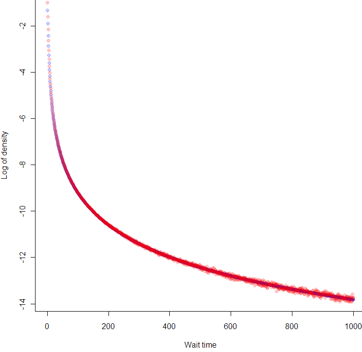
Maybe you trust my math, maybe you don’t and skimmed over the last section. Either way, let’s see how well the math matches the data. Here I’ve plotted the log of the observed (Monte Carlo) density versus what the math says it should be:
Looks like we nailed it, no? But wait, why are the blue points at the beginning of the curve in between the red points? That’s because we took the differences between points on the empirical CDF, so each density reading is really in-between the true pdf values. So far as Monte Carlo confirmation goes, it doesn’t get much better than this.
Introducing, the Unreliable Friend Distribution!
So far as I can tell, other than the hyperexponential, which is merely similar and more limited, this is a brand new distribution. Have you ever been waiting for someone, and the more they make you wait, the more you suspect they’ve forgotten about you completely? In that person’s honor, I’m calling this the Unreliable Friend Distribution (UFD).
As seems appropriate for such a distribution, the expected wait time for the UFD is infinite. Which means that no matter how late your unreliable friend shows up, you should be grateful that he came early.
The code:
# Code by Matt Asher for StatisticsBlog.com
# Feel free to modify and redistribute, but please keep this header

set.seed(943) #I remembered this time!

# Initial MC sampling
trials = 10^7
results = rexp(trials, runif(trials))

# Plot of liklihood curves for U based on waiting time
# colr = sample(colours(), 1000, replace=T)

lik = function(p, t){
	return((1 - p)^(t-1)*p)
}

# x-values to plot
p = seq(0,1,0.0001)

# Waiting times
t = 1:20

dataMatrix = matrix(nrow=length(t), ncol=length(p))

for(i in t) {
	dataMatrix[i,]=lik(p,rep(i+1,length(p)))
}

plot(p, dataMatrix[1,], col=colr[1], pch=".", cex=3, bty="n" )

for(i in 2:max(t)) {
	points(p, dataMatrix[i,], col=colr[i], pch=".", cex=3)
}

# Let's standardize the area of each curve
standardMatrix = dataMatrix/rowSums(dataMatrix)

plot(p, standardMatrix[1,], col=colr[1], pch=".", cex=3, bty="n", ylim=c(0,max(standardMatrix)))

for(i in 2:max(t)) {
	points(p, standardMatrix[i,], col=colr[i], pch=".", cex=3)
}

# Find wait time curves conditional on having waited t minutes

# We need tail probabilities, let's find them!
t = 0:1000
tailP = rep(0,max(t))
for(i in t) {
	tailP[(1+i)] = length(results[results>i])/trials
}

show = seq(1,25,1)

# Blank Plot
plot(0,0,col="white", xlim = c(0,2*max(show)), ylim = c(0, 1), ylab="Probability that your friend will have shown up", xlab="Time")

for(i in show) {
	# Normalizing the probabilies so that tailP[i] = 1
	tmp = tailP[(i+1):(max(t)+1)]
	tmp = tmp * 1/tmp[1]
	tmp = 1-tmp

	print(length(tmp[tmp<.5]))

	# par(new = TRUE)
	lines(i:(max(t)), tmp, col=sample(colours(), 1), lwd=3)


	# Find the index of the closest tmp to tmp[i]
	xloc = which.min(abs(tmp[i] - tmp))

	# Put a point where we cross time 2t on the curve
	points(i+xloc-1, tmp[i], pch=4, col="black", cex=2, lwd=3)

}


plot(0,0,col="white", xlim = c(0,100), ylim = c(0, 0.25))

t = 1:20

tmp = results[resultsi]), xlim = c(0,100), ylim = c(0, 0.25), col=colr[i], cex=3)
}

tpdf = function(x) {
	toReturn = (-x*exp(-x)+1-exp(-x))/x^2
    return(toReturn)
}

tF = function(x) {
	toReturn = (exp(-x) + x - 1)/x
	return(toReturn)
}

lengths = rep(0,1000)
for(i in 0:1000) {
    lengths[(i+1)] = length(results[results>i])
}

empericalF = 1 - (lengths/trials)
empericalf = diff(empericalF)

# Because this the the perfect size for the dots!
plot(log(tpdf(1:1000)), col=rgb(0,0,1,.2), pch=20, cex=1.3728, xlab="Wait time", ylab="Log of density")
points(log(empericalf), col=rgb(1,0,0,.2), pch=20, cex=1.3728)
Tags: fight club, Halo, unreliable friend, wait times

I confirm your math with a one-liner using version 9.0 of Mathematica:
CDF[
ParameterMixtureDistribution[
ExponentialDistribution[v],
v \[Distributed] UniformDistribution[{0, 1}]
], t][[1, 1, 1]] // FullSimplify
Nice!
Great work Matt!
Cool name.
I’ve always thought of the memoryless property of the exponential as halfway in between something that gets more reliable with more observations (the sun will come up tomorrow) and less reliable (I can get one more squeeze out of the toothpaste tube)
Interesting way to look at it! I suppose the Unreliable Friend could be made discrete and used to model your state of belief about some re-occurring event.
I remember reading (but can’t remember where!) about the idea that if you observe something with a lifespan, and are completely ignorant about the mechanism that determines its lifespan, you should assume that you’ve just wandered right in to the middle of the event. So for example, if you are told a certain bridge has taken 2 years to build so far, and you aren’t allowed to examine the bridge or check a table of completion times for similar bridges, you best (unbiased?) guess would be to say that it will be completed in another 2 years. In that sense your guess would be basically replicating the unreliable friend estimate for the half-life, based on the current wait time.
I have my doubts about this argument, especially when it’s applied to longer human events. For example, human civilization has lasted for 10,000 years, so our best guess is that it will last for another 10,000. The problem you get into is one of the anthropic principle and of observer bias, in that the probability that a random person (ie you) will stop to think, “Hmmm, what’s the probability this thing will last for another ten thousand years?” is not uniformly distributed over the life of the object.
Chris Lawn, in his book on the philosopher Gadamer (reassuring entitled ‘Gadamer: A Guide for the Perplexed’) says “What we must never forget is that we are always part of what we seek to understand” which I think sums up the dilemma of using maths to model human behaviour.
I’m just reading about the very idea you mention, which in return lead me to your blog. It’s been mentioned as either the “German tank problem” or the “Doomsday argument”. There may be other names I haven’t discovered, yet.
Anyway, nice distro!
Hi Matt,
Your sense of humor is delightful. :} So: does it make sense to provide a scaling parameter to the UFD like so:
tpdf = function(x,L) {
toReturn = (-Lx*exp(-Lx)+1-exp(-Lx))/(Lx)^2
return(toReturn)
}
tF = function(x,L) {
toReturn = (exp(-Lx) + Lx – 1)/(L^2)x
return(toReturn)
}
?
Toodles,
Alexis
Hi Alexis,
I love the idea of adding a scaling parameter, but I’m not sure if the way you’ve done it works. I changed out Lx for L*x in your code to make it run, but the pdf no longer integrates to 1. May just need a tweak…
Just a few notes:
1.Your cdf can be written handily as 1 – (1-exp(-t)) / t
2. Any mixture of DFR distributions is necessarily DFR (this is in Barlowe and Proschan somewhere, I think).
3. Your distribution results from assuming that lambda is uniform from 0 to 1. What is special about 1? If lambda is uniform from 0 to M, then M emerges as a natural scale parameter.
4. Your exposition is very nice, and insightful.