
Very interesting discussion between Ed Leamer and Russ Roberts about measuring statistical effects in the world of economics, and the often problematic desire to generalize conclusions. Here’s the link.
2010
7
May 10
Connecting R and Python
There are a few ways to do this, but the only one that worked for me was to use Rserve and rconnect. In R, do this:
install.packages("Rserve")
library(Rserve)
Rserve(debug = FALSE, port=6311, args=NULL)
Then you can connect in Python very easily. Here is a test in Python:
rcmd = pyRserve.rconnect(host='localhost', port=6311)
print(rcmd('rnorm(100)'))
6
May 10
R: choose file dialog box
Needed this one recently, it pops up a window to pick a file to be used by r, then reads the contents into myData:
myFile <- file.choose()
myData  <- read.table(myFile,header=TRUE)
5
May 10
Game of Life in R

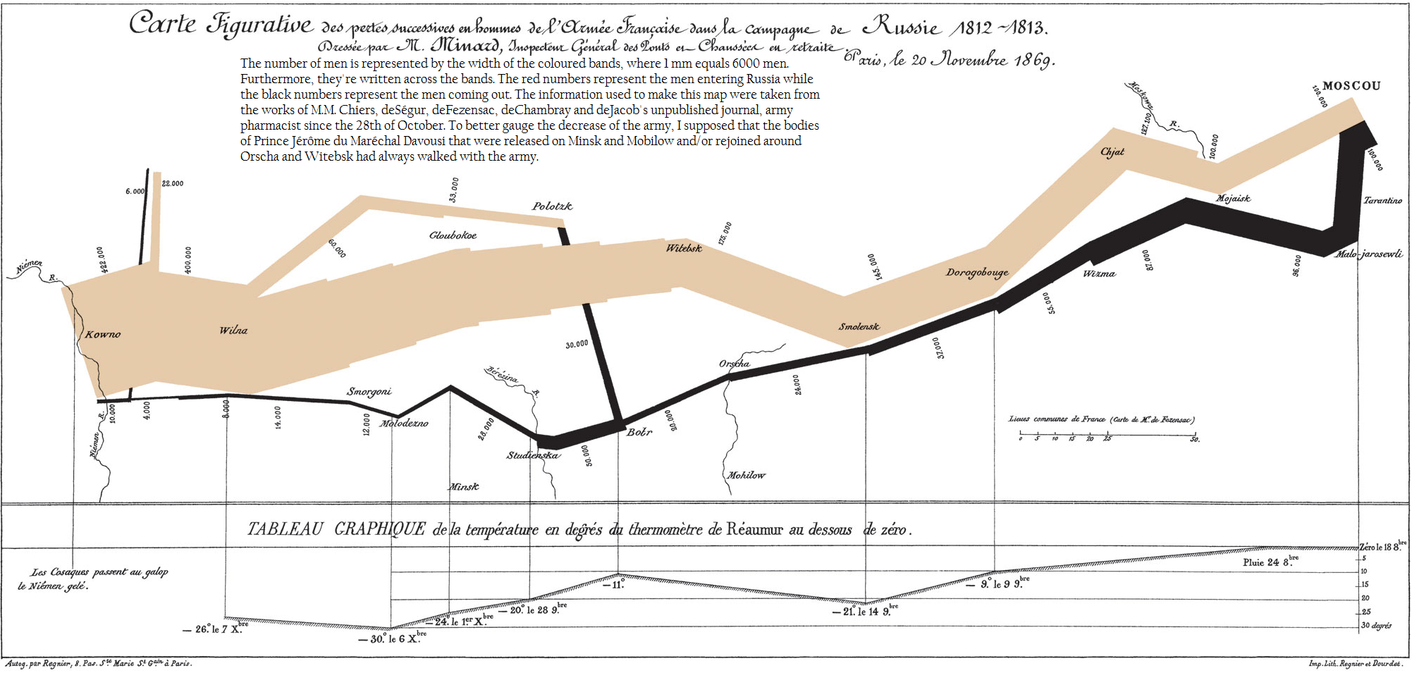
Before I decided to learn R in a serious way, I thought about learning Flash/Actionscript instead. Most of my work involves evolutionary models that take place over time. I need visual representations of change. It’s certainly possible to represent change and tell an evolving story with a single plot (see for example Tufte’s favorite infographic), but there are a lot more options when you can use animations. Flash is also object oriented, well documented with hundreds of books and websites, and has a powerful (albeit challenging to learn) IDE which helps for large coding projects.
The drawbacks to Flash are that it is way behind R in terms of statistical tools, is a closed, expensive language to work with, and dispute widespread use it might be so weak that a Apple’s iPhone might kill it.
So I picked R, with the idea that when I needed animations, I would find a way to build them. The code below is my first test of using R to generate animations. It’s a variant of Conway’s Game of Life (not to be confused with the Milton Bradley version), where single celled lifeforms live or die based on how many living neighbors they have. In my version, the rules for each cell are determined randomly, in advance of the game. The board size is fixed (see the configuration options at the beginning), whereas Conway’s version was played on a theoretically infinite grid. Green cells are “alive”, black ones are “dead”. I tried for nearly an hour to match the Black=living, White=dead scheme of Conway but couldn’t get that to work, maybe you can figure out how to do it. I re-sized the resulting animated GIF with an external program, that’s another thing I still need to figure out in R.
par(mar=c(0,0,0,0))
library(abind)
library(gdata)
library(fields)
library(grDevices)
library(caTools)
#
times = 50
myWidth = 10
myHeight = 10
#
# Set the 3D array of rules to determine transitions for each cell.
rulesArray = NULL
for(i in 1:9) {
	toBind <- matrix(sample(c(0,1),replace=T,(myWidth*myHeight)),ncol=myWidth)
	rulesArray <- abind(rulesArray, toBind, along=3)
}
#
first = T
frames = array(0, c(myWidth, myHeight, times))
for(i in 1:times) {
	if(first) {
		forFrame <- sample(c(0,1),replace=T,(myWidth*myHeight))
		first = F
	} else {
		# Convert last frame data to matrix to make comparing adjacent cells easier
		forFrame <- matrix(forFrame, ncol=myWidth)
		newFrame <- forFrame
		#
		for(m in 1:myHeight) {
			for(n in 1:myWidth) {
				adjLiving = 1 # cuz we start with array index 1
				#
				# Find out how many adjacent are living
				if(m > 1 && n > 1) {
					# Look at top left
					adjLiving = adjLiving + forFrame[(m-1),(n-1)]
				}
				if(m > 1) {
					# Look at top center
					adjLiving = adjLiving + forFrame[(m-1),(n)]
				}
				if(m > 1 && n < myWidth) {
					# Look at top right
					adjLiving = adjLiving + forFrame[(m-1),(n+1)]
				}
				if(n > 1) {
					# Look at left
					adjLiving = adjLiving + forFrame[(m),(n-1)]
				}
				if(n < myWidth) {
					# Look at right
					adjLiving = adjLiving + forFrame[(m),(n+1)]
				}
				if(m < myHeight && n > 1) {
					# Look at bottom left
					adjLiving = adjLiving + forFrame[(m+1),(n-1)]
				}
				if(m < myHeight) {
					# Look at bottom center
					adjLiving = adjLiving + forFrame[(m+1),(n)]
				}
				if(m < myHeight && n < myWidth) {
					# Look at bottom right
					adjLiving = adjLiving + forFrame[(m+1),(n+1)]
				}
				#
				# Find the corresponding rule for this cell
				newStatus = rulesArray[m,n,adjLiving]
				#
				# Update the status of this cell depending on the rule and number of living adjacent
				newFrame[m,n] = newStatus
			}
		}
#
		# Pull it out of a matrix
		forFrame = unmatrix(newFrame)
	}
	frames[,,i] <- forFrame
}
write.gif(frames, "gameOfLifeRevisited.gif", col=c("#FFFF00", "#000000") , delay=150)
4
May 10
R: directing output to file on the fly, output flushing
To start sending all output to a file, do this:
sink("path/to/filename") # Direct all output to file
print("Hi there") # Will be printed to file
sink() # Turn off buffing to file
Related to this I recently had to use:
flush.console()
This forces your console to print out any buffered content. Doing this will cost time, but if you are running a very long script and wonder if it is still alive, you might do something like this:
for(i in 10000:20000) {
	# Find the i'th prime number
	# Are we still alive?
	cat("."); flush.console()
}
3
May 10
First annual R plot replication prize

$100 to the first person who can figure out how I created this plot and replicate it. Some hints:
- It was done in R.
- There is only one underlying probability distribution involved (one “
rdist()“). - Including the “plot” statement, I created this with 3 short lines of code.
This is based on a random sampling of unstated size, so I don’t expect that your graph will be an absolute, exact match.
I’ll add $1 to the prize for every day that goes by without a winner until the end of the year. After that I’ll consider it an unsolved mystery and reveal the code I used.
Post your guesses for the code as a comment to this post. First correct answer wins. Good luck to all!
2
May 10
Anthropic principle visited (because I can visit it)

The Anthropic Principle justifies the existence of life against apparently infinitesimal small scientific odds of a life-sustaining universe. The arguments behind it can be fairly complex, but I think the most important part can be summed up very easily:
“If the outcome had been negative, we wouldn’t be around to witness it.”
In other words, if the universe had been inhospitable to human life, no one would be around to verify what came to pass. Although it is usually limited to justifying life on earth, the anthropic principle goes well beyond the cosmological. It effects how we understand any rare event which happens to happen to us.
Start with an extreme event. A fully loaded bus slides over the guardrail on a mountain pass. Ninety nine passengers die. One survives. It would hardly be surprising if that one passenger says God, and not random luck, saved her. After all, she alone survived, miraculously, while everyone else perished in a wreck which seemed destined to kill everyone.
But how do the other 99 passengers feel? Did God choose them to die, just like He apparently choose her to live? Maybe we could interview them. Oh, wait.
Take thousands of individual events, each one extraordinarily improbable, and try them out with billions of people over and over. The most likely result, the most scientifically probable, is that some people will experience extremely unlikely occurrences. If they go on to ascribe those experiences to more than just blind luck that shouldn’t surprise us. It’s only natural. But it most certainly doesn’t prove divine intervention.
Think of it this way: You, the consciousness reading these very words, are the product of millions of little events which could have just as easily gone the other way: If you mother didn’t have a soft spot for men with mustaches, if you great-grandfather hadn’t been shot down over France, if you great-great grandfather hadn’t bumped his head on that giant bottle of Sam’s Cure-all Tonic, you won’t be here today. You’re as unlikely as a tossed coin landing on its side. The universal probability bound is broken every day.
Of course the same thing goes for everyone else around you. Ten billion souls, each one coming into existence despite near impossible odds. Ten billion miracles, right? Only if you discount the stega-godzillion souls who’s coin flips landed the usual way and were never born. They are mute, silent, YouTube-impaired, invisible non-witnesses to their own bell-curve filling banality.
30
Apr 10
How many girls, how many boys?

I found this interesting question over here at mathoverflow.net. Here’s the question:
If you have a country where every family will continue to have children until they get a boy, then they will stop. What is the proportion of boys to girls in the country.
First off, there are some assumptions you need to make that aren’t stated in the problem. The most important one is that boys are just as likely as girls to be born. This is empirically false, but there’s nothing wrong with assuming it for the problem, so long as the assumption is acknowledged.
My first thought about solving the problem was to think about Martingales and stopping times, but that’s more complication than you need. If you look at it from the point of view of expectation things are simpler.The probability of having a boy first is 1/2, at which point the family stops and you have a ratio of 1 boy per 1 births. The probability of having one girl, then one boy is 1/4, at which point you have a ratio of 1 boy per 2 births. Multiplying the probabilities by the ratios and summing from 1 birth to infinity, you get an expectation of approximately 69.31% boys.
Problem is, this is the expectation for a single family. Because families who have more children (and thus more girls) contribute disproportionately to the pool of children, one family is a biased estimator for the proportion in the entire population. Douglas Zare at the above-linked mathoverflow question does a good job of working out the details for a country with an arbitrary number of families. Here is what he comes up with for the percentage of girls:

Where k is the number of families in the country, and ![]() is the digamma function.
is the digamma function.
To be true to the new motto of this site, I decided to test this out in R using a Monte Carlo method. Here is my code:
And here is the resulting graph:
Looks like a good match.

Maybe you noticed that at the beginning I mentioned assumptions, as in more than one. We are also assuming that that all of the boys and girls, no matter how old, are still considered boys and girls. All of the parents were already in the country at the beginning of the problem, and then they all started having children until they had a boy and stopped. None of these children have had any children. The process is complete, and the new generation is the last. Obviously even if parents in a country did follow the rule of "babies until boy then stop", the results wouldn't match the theoretical because at any given moment there are many families in the process of still having kids. This is where, if I were so inclined or needed a more accurate model, I would dive back into the Martingale issue and things would get messy.
21
Apr 10
R: more plotting fun, this time with the Poisson

Click on image for a larger version. Here is the code:
par(bg="black")
par(mar=c(0,0,0,0)) plot(sort(rpois(10000,100))/rpois(10000,100),frame.plot=F,pch=20,col="blue")
11
Apr 10
R frustration of the day
Whenever you take a 1 column slice of a matrix, that gets automatically converted into a vector. But if you take a slice of several columns, it remains a matrix. The problem is you don’t always know in advance how big the slice will be, so if you do this:
You'll get an error if x is 1. This creates the worst kind of bug: an intermittent one that will hide until the right (wrong?) value of x occurs. To fix the problem you need to RE-declare the slice to be a matrix with ncol=x after you take the slice.